Creating parameterized 2D airfoils with quadratic Bézier curves and Python
Before any type of shape optimization can occur, the geometry needs to be parameterized (usually…). One of the easiest ways to accomplish this is through the use of Bézier curves. For this tutorial, we’re not going to manipulate an existing geometry, rather we’re going to generate the geometry from scratch using a series of connected Bézier curves called a composite Bézier curve.
A quadratic Bézier curve is defined using three control points. The first and third point are what’s called anchor points, while the middle point controls the shape of the curve. For $$ 0 \le t \le 1 $$, a quadratic Bézier curve is defined as:
$$ B \left ( t \right ) = \left ( 1 - t \right ) \left [ \left ( 1 - t \right ) P_0 + t P_1 \right ] + t \left [ \left ( 1 - t \right ) P_1 + t P_2 \right ] $$
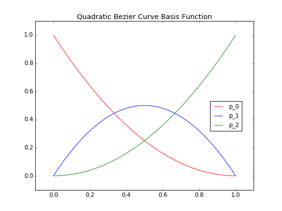
As a quick mental example, t, is a one dimensional array of values going from 0 to 1 such as t=[0.0,0.25,0.5,0.75,1.0]. As we loop through our values within t, we can see that the weighting of each control points changes. At t[0]=0.0, $$ P_0 $$ has 100% of the influence. As we cycle forward to t[3]=0.5, $$ P_1 $$ has the dominate influence. And finally, at t[5]=1.0, $$ P_2 $$ has 100% of the weighting. Below, I have plotted the quadratic Bézier curve basis function which graphically shows the influence each control point has on the curve as you progress from t=0 to t=1.
To implement this in Python we’ll have two sets of the above equation. One for the x-coordinates and one for the y-coordinates. Below is a very simple code that demonstrates what a single quadratic Bézier curve looks like. GitHub script download (here)
#------------------------------------------------------------------------------+
#
#   Nathan A. Rooy
#   Simple Quadratic Bezier Curve Example
#   2015-08-12
#
#------------------------------------------------------------------------------+

#--- IMPORT DEPENDENCIES ------------------------------------------------------+

from __future__ import division
import numpy as np

#--- MAIN ---------------------------------------------------------------------+

numPts=20                                   # number of points in Bezier Curve
controlPts=[[0,0],[0.5,1],[1,0]]            # control points
t=np.array([i*1/numPts for i in range(0,numPts+1)])

B_x=(1-t)*((1-t)*controlPts[0][0]+t*controlPts[1][0])+t*((1-t)*controlPts[1][0]+t*controlPts[2][0])
B_y=(1-t)*((1-t)*controlPts[0][1]+t*controlPts[1][1])+t*((1-t)*controlPts[1][1]+t*controlPts[2][1])

#--- PLOT ---------------------------------------------------------------------+

from pylab import *
xPts,yPts=zip(*controlPts)
plot(B_x,B_y,'b',label='Bezier Curve')
plot(xPts,yPts,color='#666666',)
plot(xPts,yPts,'o',mfc='none',mec='r',markersize=8,label='Control Points')
plt.title('Quadratic Bezier Curve')
plt.xlim(-0.1,1.1)
plt.ylim(-0.1,1.1)
plt.legend(loc=1,fontsize=12)
plt.savefig('01-basic-quadratic-bezier-curve.png',dpi=100)
plt.show()

#--- END ----------------------------------------------------------------------+
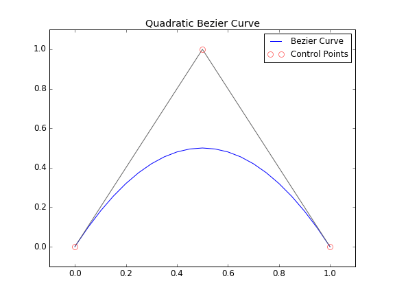
Below is an image of the final product. If we look back at the quadratic Bézier curve formula, $$ P_0 $$ is the red control point located at (0,0), $$ P_1 $$ and $$ P_2 $$ are located at (0.5,1) and (1,0) respectively.
If we animate the above script to show the progression, it becomes very easy to see how Bézier curves actually work.
At least for me, the animation really helps bring a better understanding to the underlying math. So how does this relate to airfoils, geometry manipulation, or aerodynamic design? Simple, all we need to do now is string together a series of these curves so that we can create something useful. This is what’s called a composite Bézier curve, essentially a piecewise series of individual Bézier curves lined up to form a single curve. This will allow us to start creating and manipulating complex geometry. Below is a simple script for generating a composite Bézier curve based off an arbitrary number of control points. GitHub download (here).
#------------------------------------------------------------------------------+
#
#   Nathan A. Rooy
#   Composite Quadratic Bezier Curve Example (Airfoil)
#   2015-08-12
#
#------------------------------------------------------------------------------+

#--- IMPORT DEPENDENCIES ------------------------------------------------------+

from __future__ import division
import numpy as np

#--- MAIN ---------------------------------------------------------------------+

def quadraticBezier(t,points):
    B_x=(1-t)*((1-t)*points[0][0]+t*points[1][0])+t*((1-t)*points[1][0]+t*points[2][0])
    B_y=(1-t)*((1-t)*points[0][1]+t*points[1][1])+t*((1-t)*points[1][1]+t*points[2][1])
    return B_x,B_y

def airfoil(ctlPts,numPts,write):
    curve=[]
    t=np.array([i*1/numPts for i in range(0,numPts)])

    # calculate first Bezier curve
    midX=(ctlPts[1][0]+ctlPts[2][0])/2
    midY=(ctlPts[1][1]+ctlPts[2][1])/2
    B_x,B_y=quadraticBezier(t,[ctlPts[0],ctlPts[1],[midX,midY]])
    curve=curve+zip(B_x,B_y)

    # calculate middle Bezier Curves
    for i in range(1,len(ctlPts)-3):
        p0=ctlPts[i]
        p1=ctlPts[i+1]
        p2=ctlPts[i+2]
        midX_1=(ctlPts[i][0]+ctlPts[i+1][0])/2
        midY_1=(ctlPts[i][1]+ctlPts[i+1][1])/2
        midX_2=(ctlPts[i+1][0]+ctlPts[i+2][0])/2
        midY_2=(ctlPts[i+1][1]+ctlPts[i+2][1])/2

        B_x,B_y=quadraticBezier(t,[[midX_1,midY_1],ctlPts[i+1],[midX_2,midY_2]])
        curve=curve+zip(B_x,B_y)

    # calculate last Bezier curve
    midX=(ctlPts[-3][0]+ctlPts[-2][0])/2
    midY=(ctlPts[-3][1]+ctlPts[-2][1])/2

    B_x,B_y=quadraticBezier(t,[[midX,midY],ctlPts[-2],ctlPts[-1]])
    curve=curve+zip(B_x,B_y)
    curve.append(ctlPts[-1])

    # write airfoil coordinates to text file
    if write:
        xPts,yPts=zip(*curve)
        f=open('airfoilCoords.txt','wa')
        for i in range(len(xPts)):
            f.write(str(xPts[i])+','+str(yPts[i])+'\n')
        f.close()

    return curve

#--- 11 CONTROL POINT AIRFOIL EXAMPLE -----------------------------------------+

points=[[1,0.001],              # trailing edge (top)
        [0.76,0.08],
        [0.52,0.125],
        [0.25,0.12],
        [0.1,0.08],
        [0,0.03],               # leading edge (top)
        [0,-0.03],              # leading edge (bottom)
        [0.15,-0.08],
        [0.37,-0.01],
        [0.69,0.04],
        [1,-0.001]]             # trailing edge (bottom)

#--- RUN EXAMPLE --------------------------------------------------------------+

curve=airfoil(points,16,write=True) # pick even number of points so that the leading edge is defined by a single point...

#--- PLOT ---------------------------------------------------------------------+

from pylab import *
import matplotlib.pyplot as plt

xPts,yPts=zip(*points)
xPts2,yPts2=zip(*curve)
plot(xPts2,yPts2,'b')
plot(xPts,yPts,color='#666666')
plot(xPts,yPts,'o',mfc='none',mec='r',markersize=8)
plt.title('Composite Quadratic Bezier Curve Based Airfoil')
plt.xlim(-0.05,1.05)
plt.ylim(-0.55,0.55)
##plt.savefig('airfoil-final.png',dpi=72)
plt.show()

#--- END ----------------------------------------------------------------------+
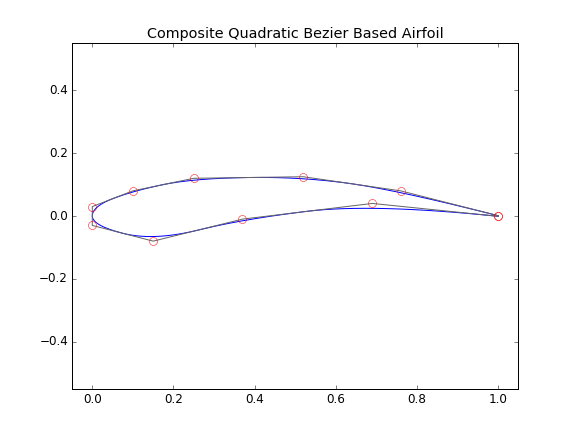
The above example is a generic airfoil featuring 11 unique control points and a finite thickness trailing edge. Now that we have covered the basics, in a future post, I’ll explain how we can use this script to optimize airfoils for a given performance characteristic.