BlenderFOAM: Open-source Fluid Based Shape Optimization

Introduction

I was recently cleaning out my closet and came across an old hard drive labeled “grad school”. After plugging it in and exploring it for a few minutes, I came across all my old thesis stuff. Seeing how this was before I started using GitHub, I figured I would post it in hopes that someone else could get some use from it. Even though it uses older versions of both Blender and OpenFOAM, the results should still be perfectly acceptable given that the equations of fluid dynamics haven’t changed much in the last hundred years.

Background

Given the ubiquity of cheap computing power both locally and in the cloud, the number of industries that deal with computational fluid dynamics (CFD) based shape optimization continues to grow. What started out as a niche skill set for aerospace applications expanded out into high high-end motorsport and naval applications. Now, CFD based aerodynamic shape optimization is a key step in the design process for every major automotive company. And if the adoption of electric vehicles continues, aerodynamic shape optimization will only become more important. The simplest, cheapest way to increase electic vehicle range is through aerodynamic drag reduction. Same thing applies to ground based shipping. A small reduction in drag across an entire fleet of trucks means massive savings overall. BlenderFOAM was my thesis project and solution to this problem. It’s based entirely on open-source software, more specifically: Blender, OpenFOAM, and Python.

OpenFOAM or Open Field Operation and Manipulation is an open-source toolbox that facilitates numerical solving and pre-/post-processing of continuum mechanics problems. Written in C++, OpenFOAM specializes in solving CFD simulations in massively parallel environments. Development of the original OpenFOAM started in the late 1980’s at Imperial College, London. Its development was initiated because of a need for more a powerful and flexible simulation platform. At the time, Fortran was the defacto standard for writing simulation code, however C++ was chosen as the programming language due to its higher modularity and object-oriented features. A distinct advantage of OpenFOAM over other black box commercial CFD codes is its complete transparency which makes it easy to modify or integrate custom written modules such as experimental turbulence models. This ease of custom development stems from OpenFOAM’s syntax which closely resembles the tensor operations and partial differential equations being solved. If anyone tells you they’re a CFD expert and doesn’t use OpenFOAM, turn around and walk away. Every solver that isn’t OpenFOAM (Ansys, STAR-CCM+, Exa, etc…) are for children.

Blender on the other hand is an open source design tool produced by the Blender Foundation and used primarily for graphics and animation. Its origin can be traced back to an in-house design tool used by the Dutch commercial animation company NeoGeo and Not a Number (NaN). When NaN went bankrupt in 2002, Blender source code was released and the Blender Foundation was formed to continue software development. Blender is primarily used for animated films and highly detailed static renderings. In addition, Blender is capable of producing interactive 3D applications and video games. Within Blender, a rich diversity of mesh creation and deformation tools are available and all accessible from the built-in python API. This enables complete automation via the terminal using batch scripts or Python. Users can also use Python to develop custom tools that can be easily implemented into the GUI. A distinct advantage of Blender is its very low hardware requirements which allows for rapid mesh deformation of high-resolution models to occur very quickly on a standard desktop computer. This lends itself very well to the task of aerodynamic shape optimization.

Geometry Parameterization

Before any shape optimization can take place, the geometry must be parameterized. Since Blender lacks support for parametric geometry, CAD files must be converted into a triangulated surface mesh and imported as an stl. Once the geometry is in Blender though, it can be parameterized using one or several different methods.

The most common mesh deformation method I find myself using is the lattice. It’s simple, easy to use, and gets the job done. The lattice mesh deformation tool (figure [1]) is Blenders implementation of a free-form deformation method. It is initiated by the creation of a 3D bounding box which is then filled with a user specified number of evenly spaced control points along each principal axis. These control points can then be maneuvered, manipulating the geometry accordingly using a volumetric B-spline function. This B-spline approach allows the lattice to have a localized impact on the geometry which spans no more than two control points in distance.

Figure 1: Lattice

Sometimes, one lattice just doesn’t deliver enough deformation fidelity and you need to use several. No Problem! Blender is a beast, and will gladly support any number of additional lattices. This enables users to create a finely tuned parametric mesh, ready for optimization. This permits optimization on different length scales which for most real world applications is a must. Seen below in figure [2], additional lattices have been implemented to increase shape control.

Figure 2: Multiple lattices

If one or more lattices fail to deliver, the next option is a cage. From the users perspective, the cage deformation tool (figure [3]) is very similar to the lattice tool. Control points are manually created and formed into a cage encompassing the geometry. This cage is free to take any shape the designer requires so long as it forms a closed surface. The control points forming this cage can then be adjusted, manipulating the geometry within. This enables a potentially large reduction in the number of control points, thus reducing the design space through intuitive placement of control points. The Blender cage system is based on work done at Pixar.¹ The cage method operates by first embedding itself to the geometry volume by solving Laplace’s equation. From this solution, the influence of each control point on the geometry is now known. Because of the global nature of elliptic PDEs, each control point has a theoretical influence on all parts of the geometry. In practice however, the influence of a control point on the geometry surface decays rapidly. An advantage of the cage method is that once it has been embedded to the geometry surface, deformations are extremely rapid, requiring only matrix-vector products.

Figure 3: Cage

The last form of geometry manipulation comes from actual point manipulation of the geometry (figure [4]). This method is basic and primitive, however in some circumstances it may prove to be the most useful.

Figure 4: Direct

Overall, Blender supports a rich environment for mesh deformation. The covered techniques can not only run in series together on a single feature, they are only a small sample of whats available to designers. And thanks to Blender’s built-in Python API, custom techniques are a simple addition.

Optimizer Performance

A simple way to measure both optimizer performance and geometry parameterization is through an inverse design challenge. Starting off with the Tyrrell 26 airfoil which used on the front wing of the 1998 Tyrrell Formula 1 car seen below in figure [5], the geometry will be subjected to a random perturbation using a lattice resulting in a completely new airfoil shape.

Figure 5: Tyrrell from 1998

The goal of this exercise will then be to recover the deformed shape back to the original airfoil in as few iterations as possible. To get a better understanding of performance, two tests will be carried using lattices of different resolutions.

Figure 6: Target (left) and deformed (right) - 4 control points Figure 7: Target (left) and deformed (right) - 10 control points

To quantify the difference between the initially perturbed airfoil and the target airfoil, a purely geometric cost function has been created. It can be seen from equation [1] below that it’s simply the squared sum of the distance between the actual and target vertices.

From equation [1], v_i are the current airfoil vertex coordinates and v_i^*, are the corresponding target vertex coordinates. The optimizers for this exercise have been assigned a maximum function evaluation limit of 1500 and a convergence tolerance criteria of 1e-03.

Figure 8: Shape matching results, 4 control points (top), 10 control points (bottom)

From figure 8 above, it can be seen that Blender and the associated optimizers are able to fully recover the airfoil geometry within a respectable number of iterations. Of note is the relative ease in which BOBYQA and NEWUOA were able to converge quickest in both a 4 and 10 dimensional space. This hints at the fact that this scenario is likely a fairly smooth, unimodal problem.

Multi-objective Airbox Design

For this test, BlenderFOAM will be challenged to optimize the performance of a Formula Ford airbox as seen below in figure [9]. This geometry was chosen because it represents one of the most common parts in the world of motorsport. Almost every vehicle features an airbox of some sort, making it a highly engineered component.

Figure 9: Formula Ford airbox

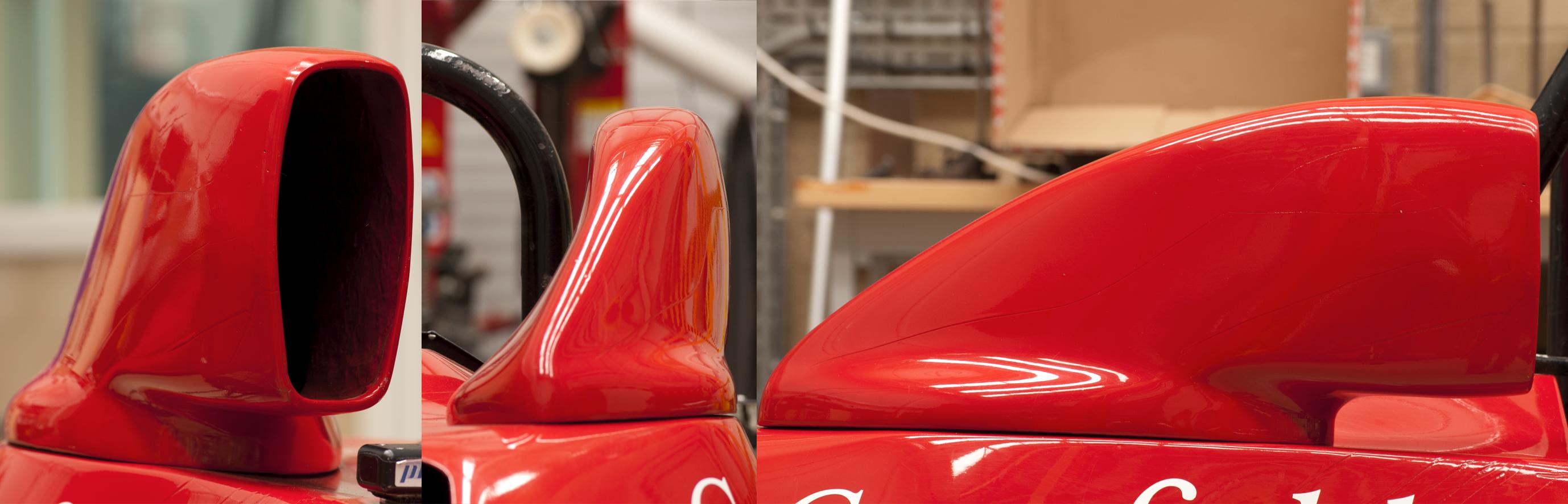
The purpose of an airbox is to deliver large amounts of air to the engine as painlessly as possible. Therefore the objective is to make the airbox as efficient as possible by minimizing the pressure loss between the inlet and outlet. The more efficient an airbox is, the easier the engine can breathe resulting in better performance.

A multi-objective approach has been used here because when optimized for purely a pressure loss improvement, the pressure distribution at the outlet can become highly uneven with a large amount of high pressure developing along the edges. For this reason, the pressure loss will be minimized while also minimizing the standard deviation of the velocity magnitude at the outlet.

Figure 10: Airbox parameterization

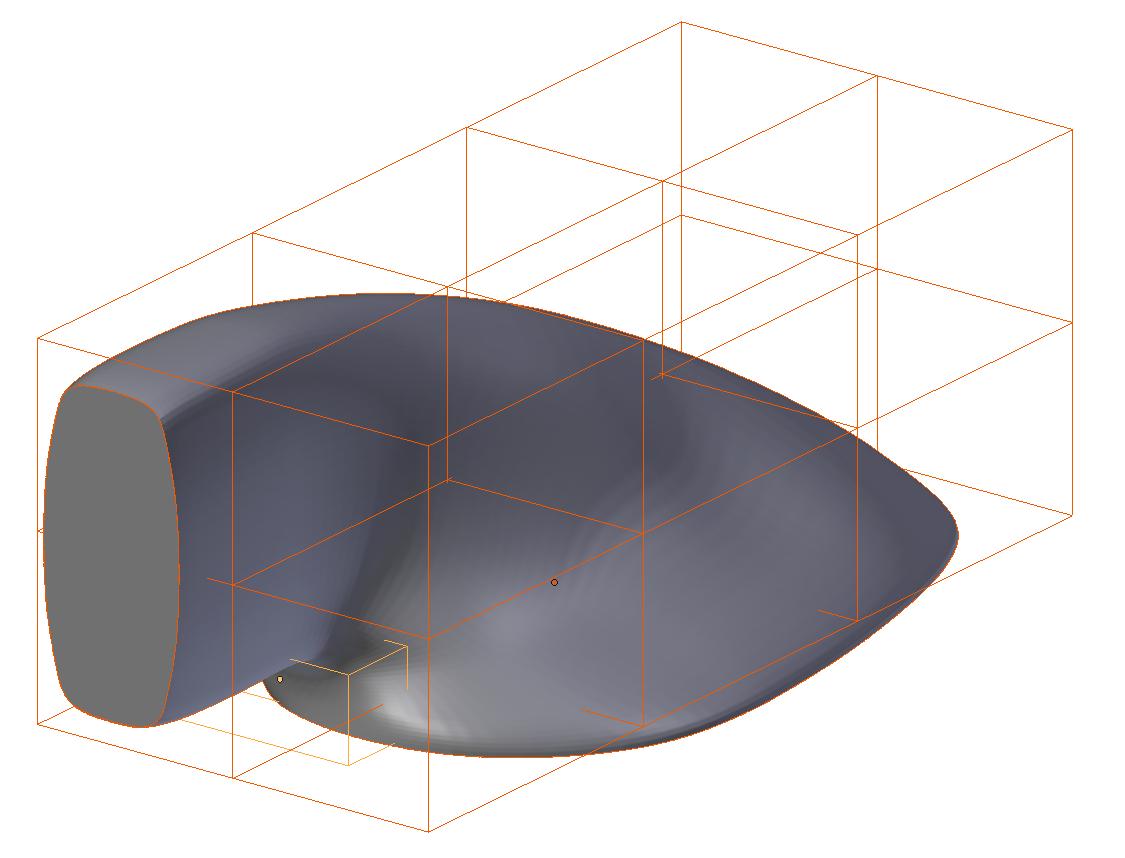
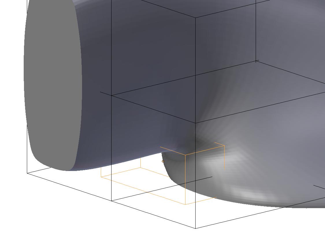
The airbox geometry was parameterized using two lattices, one for macro scale structural deformations and a smaller one was located near the neck to reduce the chances of initial flow separation. Using the simpleFOAM solver along with the SST K-ω turbulence model, the inlet has been assigned a velocity of 30 m/s (67.1081 mph) normal to the inlet plain with an outlet pressure of 0.0 Pa. Note that this setup has been heavily simplified relative to what is normally considered ideal. A setup more aligned with motorsport best practices would include optimizing across a range of inlet velocities (Reynolds sweep), inlet velocity directions, initial turbulence levels, and varying outlet pressure levels as well as external geometric constraints. In addition, simpleFOAM which is a RANS based solver should be swapped for a DES or LES based approach to better resolve small-scale, time-dependent turbulence structures. Lastly, because this was ran on my laptop and thus computationally limited, cell count was kept low at 323,480.

Figure 11: Initial velocity magnitude (left) and final (right) Figure 12: Initial turbulent kinetic energy (left) and final (right)

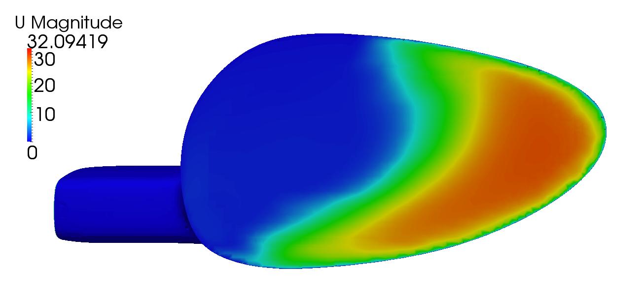
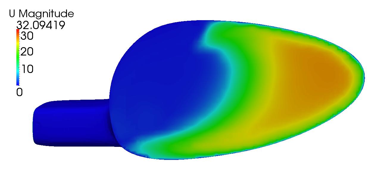
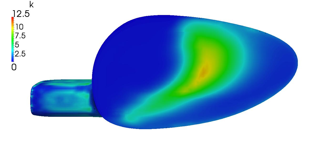
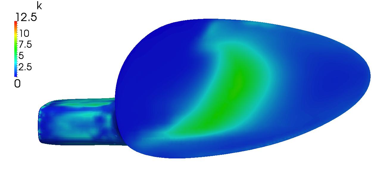
From figures [11] and [12] above, a direct comparison between the initial and optimal solution can be seen. Of interest is the improvement in flow distribution as seen by the velocity magnitude. To further improve flow uniformity, additional fidelity is needed. This could be accomplished by adding more control points however the solution would become increasingly more expensive. A cage parameterization would be ideal.

Below the solution convergence can be seen from both the velocity distribution and pressure loss perspectives.

Figure 13: Solution convergence for pressure loss (left) and flow uniformity (right)

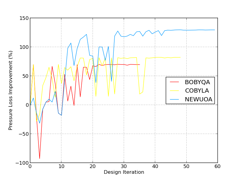
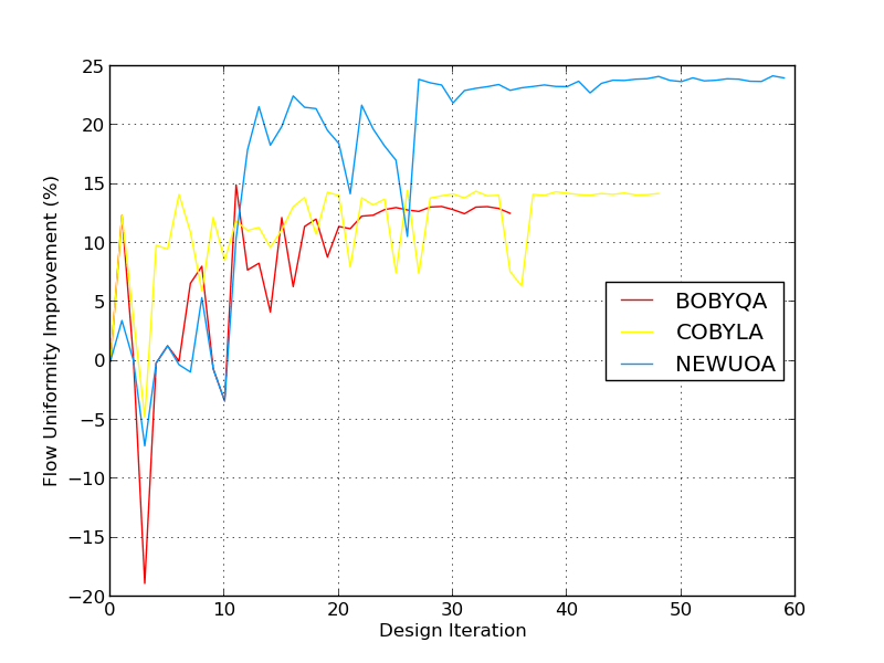
Lastly, the distribution of solutions can be seen below in figure [14]. A wide variety of responses were created from the optimizers with the majority succeeding in improving the performance of the airbox. Of interest is the diverse range that NEWUOA creates in its search for the optimum. This is a positive attribute in that, the search space is completely and evenly filled except near the optimum where there is a concentration of designs.

Figure 14: Airbox design canidates

The initial airbox and the NEWUOA optimized design can be seen below in figure [15]. One can easily see the differences between the initial and optimized designs.

Figure 15: Optimization results - initial (left), final NEWUOA solution (right)

Although this platform found substantial performance improvements for this Formula Ford airbox, one has to remember that this is a single wall structure and any geometric adjustments will impact both internal and external flow properties. The current optimized design may provide better internal flow conditions but it might also adversely impact the external drag of the vehicle rendering it useless.

Conclusion

Overall open-source based aerodynamic shape optimization if used correctly can be an extremely powerful design tool. Its performance has been proven, and its application has been demonstrated. Instead of paying tens of thousands of dollars for a single seat of commercial black box mystery, one could simply clone [this repo] and begin optimizing!

Acknowledgements

Special thanks once again to Paolo, and Eugene at Engys for helping me while I completed my thesis.