Visualizing One Hundred Years of Cincinnati Maps

Introduction

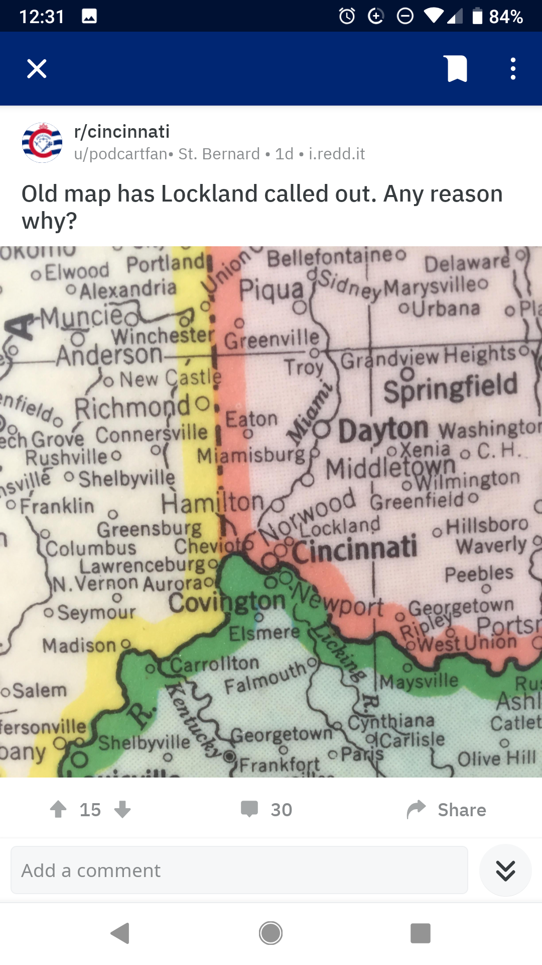
A while back, someone posted on the Cincinanti subreddit an interesting mapping artifact. I didn’t know the answer to the question, but it got me thinking about what else has changed over time in Cincinnati in regards to maps and names? Luckly the Cincinnati Public Library Digital Archives has a wealth of information on just this topic.

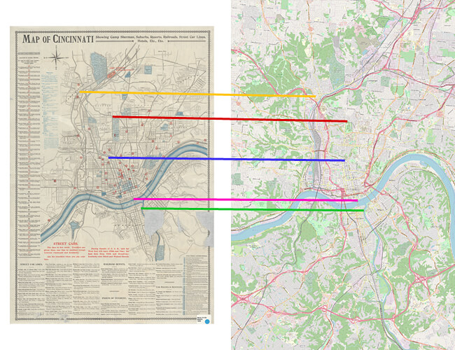
I ended up downloading about a dozen maps ranging from as early as 1815 to as recent as 1900. I then georeferenced these maps against a single modern map using known commonalites such as prominant intersections and landmarks. This standardization process, although a bit tedious, results in a final product which allows for a true apples to apples comparison. At this point, the maps can be stacked on top of each other and visualized. Below is the end result of this (make sure to go fullscreen!). For more on the technical details, see the methodology section below.

Note: On mobile devices, the side-by-side plugin I'm using with Leaflet seems to work best when both thumbs are used to navigate/zoom rather than just one...

Final Thoughts

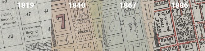
After a few weeks of georeferencing these maps, I noticed a few noteworthy observations, the first of which was the gradual development of Washington Park and surrounding areas. Back when Cincinnati was just a small town, the decision was made to build a cemetery on the northern most edge of the city. At the time, this land would have represented the boundary between civilization and untamed wilderness. Fast forward almost two hundred years and the city has not only expanded out far beyond these initial cemeteries, but they have become the focal point of present day downtown! Today, only a few headstones remain while the rest has been replaced with grass, a dog park and Music Hall.

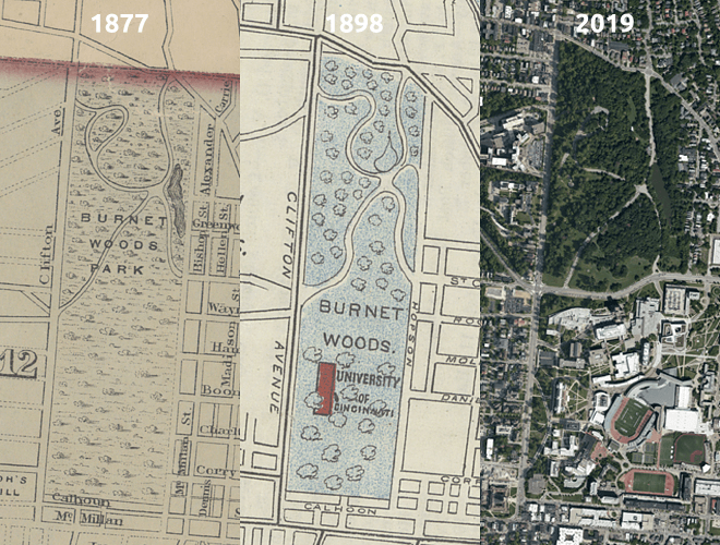
Another interesting observation centers around Burnet Woods and the University of Cincinnati. I knew that UC was founded in 1819, however I never knew that the land it was built on was taken from Burnet Woods. It appears that the UC’s campus has shaved off nearly half of the original Burnet Woods.

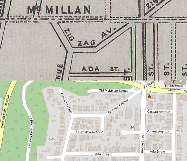
Lastly, and most importantly is the tragic renaming of Zig Zag Avenue to Fairview Avenue sometime between 1898 and today. For starters, Zig Zag Ave is the name every other street wish it had. Seriously, not even Lombard St. is good enough for a name like that. Fairview Ave is the kind of thoughtless generic street name that belongs out in suburbia, not Clifton. What kind of monster thought this was a good idea?

Hopefully this can serve as a useful tool for anyone doing historical research or maybe just a fun way to explore this great city. If anyone stumbles across some high resolution maps, feel free to reach out and I can add them.

Thanks for reading, and bring back Zig Zag Ave!

Acknowledgements

Special thanks to Diane at the Cincinnati Public Library for going above and beyond with helping me aquire the high resolution version of these maps. 🙌

Methodology

First step in turning the old map scans which come in the form of raster image data into something usefull is to standardize them somehow. Since I had no idea what datum or coordiante reference system (CRS) they were originally created around I couldn’t do a direct transormation. This meant I had to put them through a round of georeferencing which is basically just the cartographers version of image registration. Since my end game was to present these maps over the internet, I knew that the final CRS would need to be the web Mercator projection aka EPSG:3857 which is based on the WGS 84 datum. This is the same system that most web mapping applications such as Google Maps, OpenStreetMaps, and Bing Maps use.

With the CRS sorted out, all that was left was to calculate the required transformation which would take take the scanned raster map images and translate them to web Mercator coordinates. This was accomplished through the use of thin plate splines (TPS), delaunay triangulation, and bicubic interpolation.

As the name implies, TPS refers to the imaginary situation in which a thin sheet of metal is undergoing a series of bending operations. The goal with TPS is to maximize the smoothness (or minimize total bending energy) of the final metal surface, because it’s this deflection in the z-axis (orthogonal to the plane) which will control the deformation of our image. Because our images will be deformed in both the x, and y directions, we will need to solve two instances of the TPS equations.

To begin, let \( \{s_j\},\{t_j\}, \; j=1,...,n \) represent the landmarks (x,y coordinate pairs) from the source (\( s_j \)) and target (\( t_j \)) images. Below is an example of the process. Note that only five coordinate pairs are displayed for visualization purposes. In reality, most maps require at least ~50 coordinate pairs while others require over 300 coordinate pairs.

Figure 1: Source (left) and target (right)

The end goal is to find a smooth function such that: \( f : \Omega \subset \mathbb{R}^d \to \mathbb{R}^d \) that satisfies the interpolation conditions:

$$ f \left( s_j \right) = t_j \qquad \text{for} ; j=1,…,n \tag{1} $$

Once these conditions have been met, the situation becomes one of minimization.

$$ \mathcal{T} \left| f \right| = \sum_{j=1}^n \lVert f \left( s_j \right) - t_j \rVert $$

where \( \lVert \cdot \rVert \) represents the Euclidean norm. Depending on the spatial distribution of the landmark coordinate pairs, the smoothness of the interpolated surface can vary drastically. To help improve the smoothness of the surface, a gradient based regularization term can be added at the expense of losing the initial interpolating conditions from Equation [1]. The addition of this regularization term produces the following objective function:

$$ \mathcal{T} \left| f \right| = \sum_{j=1}^n \lVert f \left( s_j \right) - t_j \rVert + \lambda \int_\Omega \lvert \nabla^m f \rvert^2 d\Omega \tag{2} $$

where \( \Omega \) represents the domain of the image. This objective function \( f \) is what’s known as a polyharmonic spline, which when \( m=2 \), becomes a special case known as the thin plate spline. The weight of the regularization parameter is controlled using \( \lambda \geq 0 \) (higher values of lambda result in a smoother surface). In two dimensions, the thin plate spline minimizes the following objective function:

$$ \mathcal{T} \left| f \right| = \sum_{j=1}^n \lVert f \left( s_j \right) - t_j \rVert + \lambda \iint \left[ \left( \frac{\partial^2 f}{\partial y^2} \right)^2 + 2 \left( \frac{\partial^2 f}{\partial y \partial x} \right)^2 + \left( \frac{\partial^2 f}{\partial x^2} \right)^2 \right] dx dy \tag{3} $$

Equtation [3] represents the closed form solution to the thin plate spline interpolation which was originally developed by Dunchon¹ in 1977. It wasn’t until 1990 when Whaba² proved the existance of a unique minimizer as seen below³:

$$ f \left(x,y \right) = a_1 + a_2 x + a_3 y + \sum_{j=1}^n w_i U \left( \lVert P_i - (x,y) \rVert \right) \tag{4} $$

Equation [4] represents the combination of an affine and non-affine transformation. In most texts, the non-affine portion: \( \ U (r) = \frac{1}{8 \pi} r^2 \log r^2 \), is often simplified into Equation [5] because the coefficient \( \frac{1}{8 \pi} \) is dissolved into the weight variable \( w_i \).

$$ U = r^2 \log r^2 \tag{5} $$

Since the non-affine portion of Equation [4] is a function of radius, it represents the dominate influence of deformation while in close proximity of the control points. Further away from the landmark locations, the strength of the non-affine portion (Equation [5]) diminishes towards zero. This results in the affine portion of Equation [4] exerting more influence at the extremities of the image.

Now that the transformation between the source and target can be computed, the next step is to resample the pixels. Because the images we will be dealing with come from a scanner or other digital source, each pixel represents a discrete RGB tuple point in gridded two-dimensional space. unfortunately after the TPS transformation has been applied, the pixel locations become stretched and skewed into an unstructured mess. The task at hand is to now interploate these scattered RGB tuples back onto a structured grid so they can be used like a normal image. More specifically, we want to interpolate the RGB values from the displaced source image pixels onto the exact (x, y) pixel grid of the target image.

Figure 2: Pixel resampling

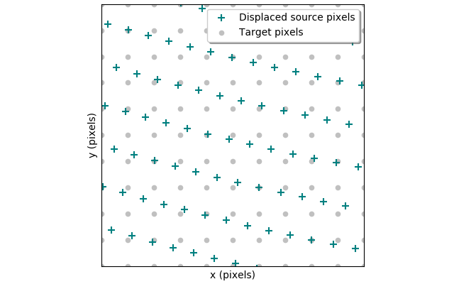
Unlike the TPS transformation which I had to code from scratch, resampling is a faily common exercise so I was able to use the built in function griddata found in SciPy. The griddata function first generates the delaunay triangulation across all of the displaced source pixels using Qhull

. Figure 3: Delaunay triangulation

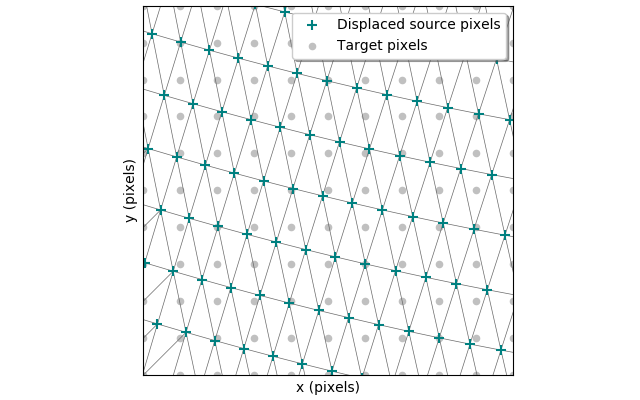
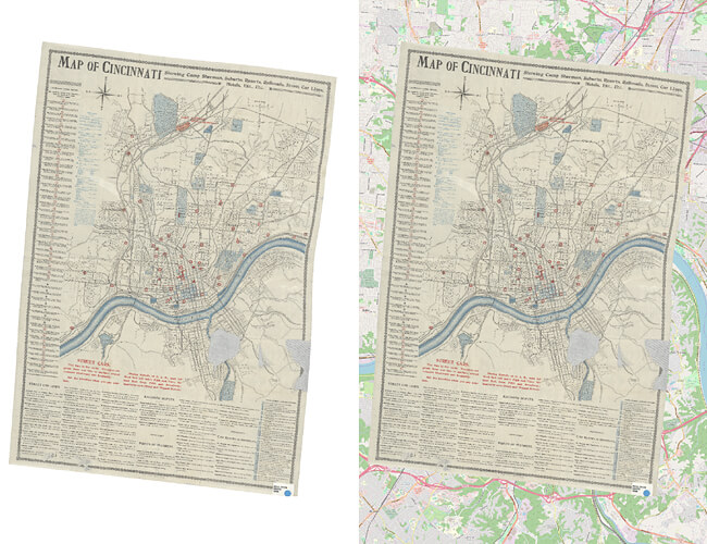
Once the triangulation has been generated, a piecewise cubic Bezier polynomial is fitted to each triangle using a Clough-Tocher scheme.^{4, 5} Since the interpolant is guaranteed to be continuously differentiable, the gradient can be chosen so as to minimize the interpolating surface curvature. The gradient is minimized using a global scheme.^{6, 7} After the resampling has been applied, an example of the final map can be seen below.

Figure 4: Final transformation

If you’re interested in georeferencing images for yourself and don’t want to start from scratch like I did, QGIS has a very nice georeferencing plugin.